Depending on the conditions prevailing in an aquifer, the water may be stagnant or moving. Usually, the water flow is of the order of a few meters per day. In many cases, we are interested in knowing the direction and speed of this flow. E.g.:
- To calculate escapes from an aquifer.
- For the calculation of the water balance.
- To assess the pumping potential of an aquifer.
- To estimate the extent of water pollution in an aquifer.
For one-dimensional flow (at the x-y plane) we can use Darcy’s law to estimate the specific flow qx
Darcy’s Law: The specific flow is linearly proportional to the hydraulic conductivity K and the hydraulic inclination.


qx = Specific Flow. t is the flow (Q) per unit area (A). It has speed dimensions, usually m/day.
K = Hydraulic conductivity. A factor that depends on how easily water passes through the soil formation. It has speed dimensions, usually m/day.
dh/dx= hydraulic gradient. Simply put, how abrupt is the difference in hydraulic height between the two positions. Dimensional.
It exists except because the direction of flow is where the hydraulic height decreases (negative hydraulic inclination).
Flow velosity
The specific flow rate qx means flow rate per unit area perpendicular to [m3 / s] / [m2], so its unit of measurement is unit speed [m / s]. The specific flow rate qx does not correspond to the flow rate. This is because the surface unit includes soil grains and gaps. But the flow is only through the gaps. So the flow velocity through is:

Where n is the porosity of the soil formation.
Example: Losses from Lake A (left) feed Lake B (right). The distance between them is 3.5 km. The water level in Lake A is at +1100 m and in Lake B at +1060 m. K = 12.5 m / day and n = 15%.
Calculate the specific flow rate (qx) and the flow rate through the pores
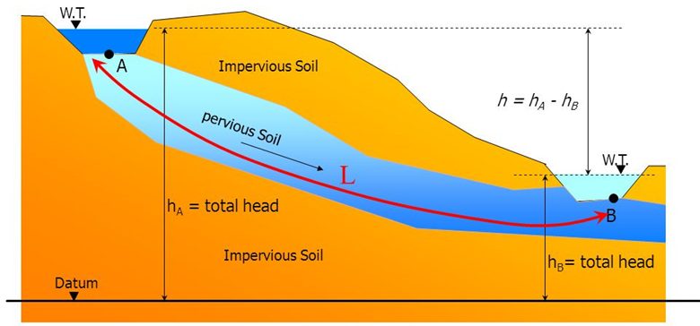
Hydraulic gradient: – dh/dx=-(1060-1100)/3500=-(-40)/3500= 0.0115
Specific discarge q=-Kdh/dx=12.5×0.0115=0.143 m/day
u_x=q_x/n=0.143/0.15=0.95 m/day
6.3.3. Aquifer discharge to the sea
Aquifers in coastal areas often have escapes to the sea. The image below shows the thermogram of a coastal area. In red, the area where water flows from an aquifer that has underground escapes to the sea stands out. Generally, depending on the season, aquifer water is either warmer or colder than seawater.

Exercise: The figure shows the characteristics of an aquifer.
– Average thickness at the outlet 3 m
– Average aquifer width: 1.5 km
Calculate the volume of water flowing to the sea

Hydraulic gradient dh/dx=2/1000=0.002
Specific discharge qx = 40 x 0.002 = 0.08 m/day
Escapes Qδ = 1500 x 3 x 0.08 = 360 m3/day
What is the velocity of water flow in the pores? Assume n=30%
u_x=q_x/n=0.08/0.30=0.27 m/day
6.3.4. Πιεζομετρικοί χάρτες
Piezometric maps show the hydraulic height at the aquifer. They are constructed using measurements of the height of the free surface of the water in monitoring wells.
Isopiesometric curves: are the curves of equal hydraulic height. In well aquifers the hydraulic height coincides with the altitude of the aquifer
